Microsoft Excel: the office staple with endless opportunities and challenges.
As a beginner, Excel is great for collating and calculating small data sets, but when your work becomes more complicated, and you get into the depths of data manipulation, the cracks can start to show.
Users often need help with error control, cross-team collaboration and automation processes. Sometimes, being a whizz at basic keyboard shortcuts isn’t enough.
It helps to invest in proper training to learn about simplifying processes, making efficient calculations, and finding those all-important solutions. This will save you time in the long run, especially when project deadlines and data reports start creeping up at the end of the financial year.
That said, there are some tweaks you can make to your daily use of Excel to reduce the margin of error in your projects. Here are some tips and tricks.
Customising the Excel Interface
Core to all Microsoft software is the ribbon at the top of the program which enables functionality. However, did you know you can personalise it to your tastes and workflow?
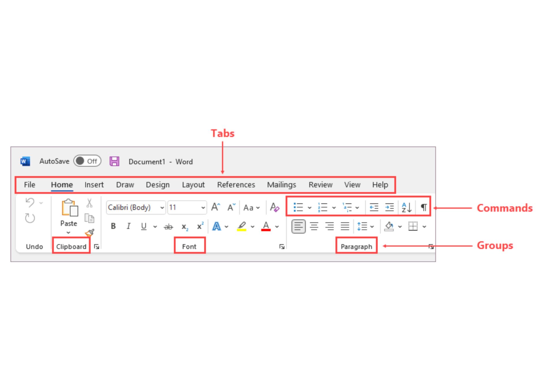
Enhance your productivity by hiding or unhiding the ribbon and commands less often used, and by arranging tabs and commands in your preferred way.
Found a ribbon set-up online that you like? Excel even has the functionality to import a downloaded ribbon.
For example, you might use PivotTables and images frequently, and dislike the extra navigation from the home tab to insert them into your spreadsheets. Simply right-click the ribbon, select personalise ribbon and format it by moving commands as you desire.
Moreover, setting default templates for regular tasks can seriously improve your workflow. Whether you’ve made your own calendar, invoice or budget template, or used one of Microsoft’s own, be sure to save it as a template for the future.
- In the save as type box, click template.
- In the save in box, select the folder that will store the template (C:\Users\<username>\AppData\Roaming\Microsoft\Templates).
- In the file name box, type book to create a workbook template, or sheet for a worksheet.
- Name the template.
- Save and close.
By setting up custom templates and a personalised ribbon, you can rest assured that your team will shave time off their daily tasks with formatting options that suit their workflow, streamlining efficiency and increasing the range of uses Excel can assist your company with.
Utilising Advanced Excel Functions
Microsoft Excel has several hidden features that can change the way you find and display your information and datasets. Some useful functions include VLOOKUP, INDEX-MATCH and PivotTables.
VLOOKUP
VLOOKUP is a search function ideal for finding a designated value or range in a large dataset. The ‘V’ in VLOOKUP stands for ‘Vertical’ and makes it clear that the function searches downwards in a column. VLOOKUP is ideal for finding values in the same row from a corresponding column.
The formula below retrieves an approximate or exact value of the data you wish to find.
=VLOOKUP(lookup_value, table_array, col_index_num, [range_lookup])
- lookup_value is the cell you want to search for in the first row.
- table_array are the rows you want to search from. One of these should have the value you are looking for.
- col_index_number is the column these rows belong to.
- [range_lookup] is an optional feature to specify if you wish Excel to return an approximate or exact match, indicated as 1/TRUE, or 0/FALSE respectively.
For example, finding an employee’s name within a table of employee information, where A is employee IDs and B is employee names, is as simple as using the following formula:
=VLOOKUP(“Employee ID”, A2:B10, 2, FALSE)
INDEX-MATCH
The INDEX-MATCH formula is a more advanced search function than VLOOKUP as it enables vertical and horizontal searches.
INDEX-MATCH combines the INDEX formula, used to retrieve a value when supplied with a row and column number, and MATCH, which can find the position of a data entry in a range.
The process works as follows:
- INDEX requires numeric positions in a data range
- MATCH can find those positions within the data range and is nested inside INDEX.
- MATCH can therefore find both the X and Y (or, horizontal and vertical) columns for INDEX to operate.
For example, this horizontal and vertical MATCH formula is:
=INDEX(First_DataCell_in_Table:Last_DataCell_in_Table, MATCH(Result_Cell, First_Cell_of_TableColumn:Last_Cell_of_TableColumn, 0), MATCH(Result_Cell2, First_Cell_of_TableColumn2:Last_Cell_of_TableColumn2, 0))
[NOTE: 0 is inserted to match the exact value]
INDEX-MATCH is helpful when identifying specific data results with many variables, such as the total sales by an employee in a certain month.
PivotTables
PivotTables are powerful tools for data analysis. They can calculate, summarise and analyse complicated data, and provide options for comparisons and visualising patterns and trends within your spreadsheet. But they can be tricky things to set up, and many users face challenges with refreshing data or customising the layout.
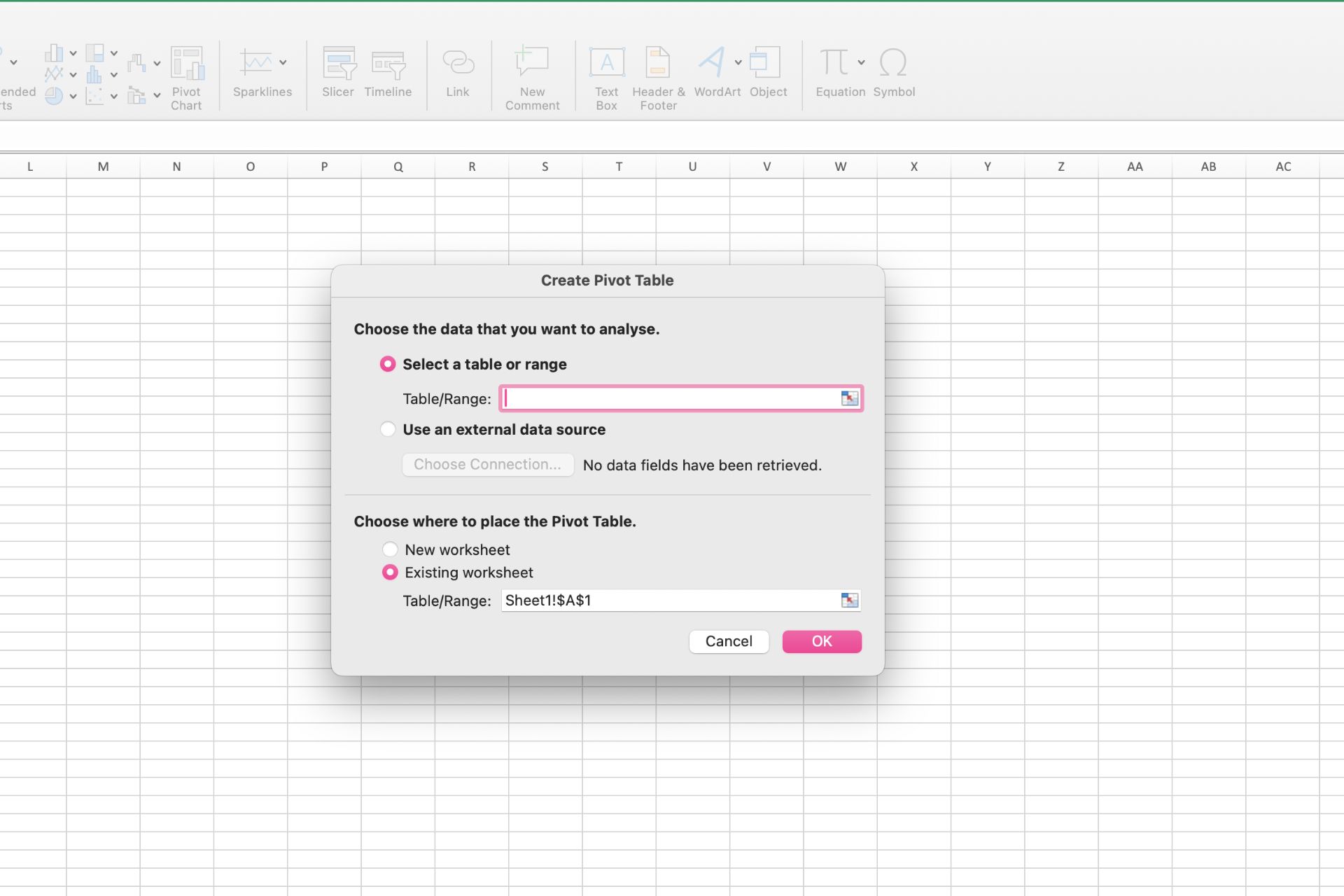
The most important tip for PivotTables is to ensure your data columns are clean. This means the table is organised with a single header row and may involve creating a separate table from your big data.
All you then need to do is select the cells you want to turn into a PivotTable, select insert > PivotTable and choose where it will be located.
PivotCharts allow your table to be easily represented as graphs. With a plethora of charts to choose from, your data is sure to be understandable by your audience.
Automating Repetitive Tasks
Are you tired of creating the same report every month? Wishing for a shortcut to formatting content? Fortunately, Microsoft Excel contains automation tools that will help you do just that.
Macros are the main automation tool to replicate repetitive tasks. They are a set of actions you create that can run as many times as you desire. When creating a macro, your mouse clicks and keyboard strokes are recorded and remembered, with the opportunity to edit and alter later.
So that monthly report that drives you up the wall? Create it once and macros will format the data fields for you, every time.
Macros are found in the hidden developer tab, so first you must open the tab by customising your ribbon. Then, hit record in the coding group, type a name of choice, and perform the actions you wish to automate on your worksheet. Stop recording when you’re finished, and voilà! You have a macro shortcut!
Now, whenever you need to use the function, go back to the developer tab, select the desired macro in the macro name box, and watch everything you recorded realise itself.
Data Validation and Conditional Formatting
Applying certain rules to your worksheet is another time-saving feature which can also reduce the chance of error.
The data validation function (located in data > data validation) restricts the type of data or values one can enter. Usually, this is with predetermined options in a drop-down list.
First, select the cells for the data validation rule. Then move to the settings tab, and under allow, select a type of input your data must take the form of, such as whole numbers, decimals, time, list or dates. Write an input message and error message. This way, if any of your team members pick up the spreadsheet, they’ll easily be able to follow along.
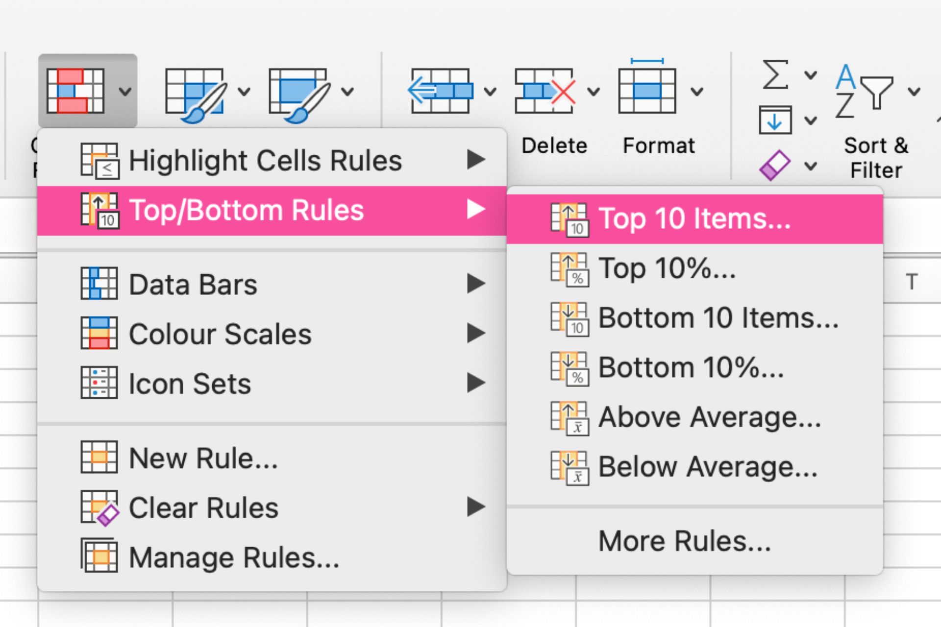
Or maybe you’d rather others clearly observe apparent trends in your Excel sheets through colour. Your boss wants to know the top monthly expenses, but there’s a long list of products the company buys, so highlighting it yourself will take too long. This is where conditional formatting for data visualisation comes in handy.
Select the cells, go to home > conditional formatting. Under the drop-down option top/bottom rules, select top 10 items. You will notice sorting occurring immediately. From there, in the pop-up window, choose how many values you want to be highlighted and their formats.
Integration with Other Tools
Gone are the days when emailing files for collaboration led to multiple outdated versions and confusion amongst office teams. Microsoft Excel is available on web browsers through OneDrive, for that added security in case your laptop crashes before saving. OneDrive updates any changes live, so there’s no risk of duplicate files.
Like any app in the Microsoft Suite, Excel connects seamlessly to SharePoint. If your team uses SharePoint, upload the spreadsheet to a page, and those with access to the SharePoint dashboards can work in real time together.
Power BI is another business software Excel files integrate easily with. Microsoft Excel is available on the Power BI home page, and from there, you can upload and visualise your workbook on Power BI. If you work from OneDrive, there are add-ins users can install to connect the gap between Excel, OneDrive and Power BI.
Level up your Excel Game Today
Don’t let the technical formula and mathematics jargon dissuade you from becoming a Microsoft Excel professional. From this article alone you have learnt about conditional statements that can assist in error checking your data, insights into maximising your personal productivity and advanced functions to speed up repetitive activities on Excel.
Practice makes perfect, and every minute spent applying these skills is a step towards greater confidence with Microsoft Excel.
Continue to master your Excel skills with our expert tips available in Priority Management’s broader Microsoft 365 training. From Microsoft Excel beginner courses to ways to upskill your number-crunching abilities, check out what Priority Management can do for you and your team today!